

September 22, 2020
The summer lull is over, and I am back. Really back. This time, I decided to go all the way back to my roots and focus on something that I have held dear for a very long time: Fourier series. Anyone who has come in contact with signal processing and its applications to communication systems knows that Fourier Series, and its derived cousins Fourier transforms, discrete, discrete-time, fast, and Z-transforms, warts and all, are indispensible tools in making sense of how signals behave in systems. It's also probably the reason why I was glad I didn't sleep through high school math classes when my teachers talked about imaginary numbers. Anyways, more on that later. I don't want to give a boring lecture on Fourier series. This is a fun blog, after all, so let me begin by going back...
Tell me what you see in the following graph:
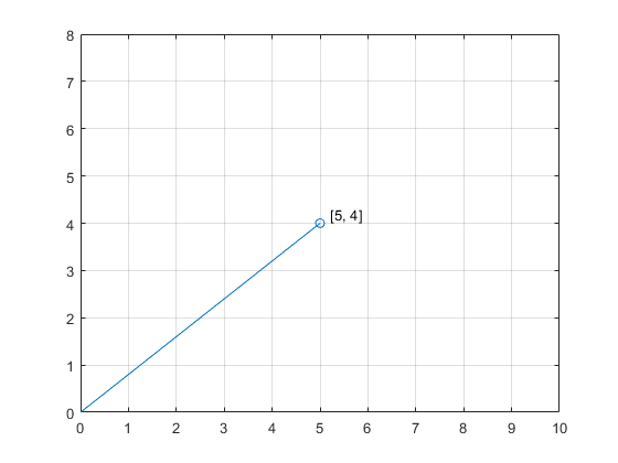
It's a vector whose head is at the origin, and the tail is at point P(5, 4). If you paid attention in grade school, the point P having that coordinate would mean that you reach to that point by starting at the origin, (0, 0), and traversing 5 units in the positive x-direction and then 4 units in the positive y-direction to complete the journey. Pretty simple, huh?
But, let me dissect the previous paragraph just a little bit, because what you've learned in school is a very, very, very simplified version of what's really going on. You see, before you begin the journey, you should know the world you are in. The world here is the 2D Cartesian plane, but Euclid did it better (sorry Monsieur Descartes!). The generalized term for the 2D Cartesian plane is the R^2 Euclidean space, which is a subspace of the R^2 inner product space which in itself is a subspace of the R^2 vector space. If all that is making your head dizzy, just note that you can have vectors in the R^2 Euclidean space that add/subtract/scalar multiply component by component and doing inner products between any two vectors is a-ok. The inner product in the Euclidean space is the dot product, which is basically the sum of the products of components of the two vectors. Anyways, the keyword here is "component". What is a component? Like making your favorite cake, a component is an ingredient that makes the cake. However, unlike ingredients to a cake recipe, you are free to make whatever vector in the Euclidean space as the component. Making the [5, 4] vector a component for the Euclidean space is totally fine. This means to make a [10, 8] vector, you just take 2 copies of the [5, 4] vector and there you have it. But, making the [5, 4] as your component in this vector space is like making the "cake" as the sole ingredient in your cake recipe. Sure, technically you are correct, but what's the use? How many "copies" (fractional and negative copies are allowed) do you need to make the [3, -1] vector, say, from your [5, 4] vector component? And if that is not possible, how many more components do you need? And what are they?
You see, things are not as simple as it seems when it comes to making components. If you want things to be useful, you would need a complete set of components whose number of copies required to form the resulting vector also form the coordinate system for such vectors created. In order to achieve this, you would need components that are:
The unit-length-ness of the basis vectors seem reasonable. But, you may wonder, why orthogonal? Well, when you are combining ingredients to make your cake, you don't want to add two tbsp's of butter confidently in the batter and then add 1 tsp of salt, only to realize that your butter was already salted, so in reality you added more than 1 tsp of salt, and now your cake is more savory than sweet. Orthogonality means that the direction of one vector is completely independent of the other, so when you are combining one vector in one direction, you are not inadvertently adding to the direction of the other.
If you can find such components, they would be called "basic vectors" in the Euclidean space. And if you gather the complete set of "basis vectors", they are called an "orthonormal set" to your vector space. You can then create any vectors in the space from the basis vectors in the orthonormal set (aka the orthonormal set "spans" the vector space), and without breaking a sweat as well, since the number of copies of the corresponding basis vectors form the coordinates of the resulting vector. The number of basis vectors in the orthonormal set is also the dimension of the Euclidean space.
For example, for the vector we are looking at:
If we make our basis vectors to be [1, 0], which I call i-hat, and [0, 1], which I call j-hat, then we can form [5, 4]. Remember we add/subtract/scalar multiply component by component, so: [5, 4] = 5[1, 0] + 4[0, 1]. We need 5 copies of i-hat and 4 copies of j-hat, which just so happens to form the coordinates of P, the tail of our vector, P(5, 4). Isn't that convenient!
In fact, you can verify that our basis vectors i-hat and j-hat can be combined in any copies where the scalar multiple is a real number (which is the field of our Euclidean space, by the way) to form any vector in the vector space! So {i-hat, j-hat} forms an orthonormal set. Note that i-hat is the unit vector along the x-axis, and j-hat that along the y-axis, so they are both unit length and are orthogonal to one other. This also means that the R^2 Euclidean space has 2 dimensions, as it should be.
It might seem that I have just stated a bunch of obvious facts, and are now wondering how any of that can be useful. Here, I start to "take apart" things. Just as you can combine basis vectors by the appropriate copies to make a resulting vector, you can also do the reverse--take the resulting vector apart and focus on one of the components: how many copies of that basis vector were needed to make the final vector? It's like eating a cake and then wondering how many cups of flour were used to bake it. Certainly useful if your friend is not willing to share with you the recipe, but it's not that easy or trivial now is it? This is where projections come in.
The projection of a vector along some other vector is another vector, that is parallel to the "other" vector in which you are trying to project onto, that forms the "shadow" of the original vector. For example, the projection of [5, 4] onto [1, 0], the i-hat, is [5, 0]. Why? When you are casting a shadow of [5, 4] along the x-axis where i-hat lies, you get the "x-direction", so to speak, of the original vector preserved but the projection would completely ignore the component along the y-axis, as expected. Similarly, the projection of [5, 4] onto [0, 1], the j-hat, would be [0, 4].
There's too much to explain, but if we are projecting a function f(t) with period T onto another one with the same period, say g(t), here is how we do it, assuming those functions are in an inner product space where projections are defined.

Where g*(t) is the conjugate of g(t). When we talk about functions here, we are assuming they are complex unless otherwise stated.
You have a circle with radius 1, and a dot is traversing along the circle. What would its path look like?
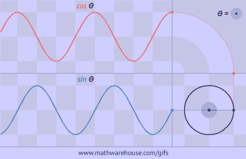
In the above animation, θ is the angle between the radius from the center to the dot's position and the radius from the center to (1, 0). The function cos(θ) then measures the horizontal displacement of the dot as it traverses along the circle, and the function sin(θ) measures the vertical displacement.
How fast is the circle going? From grade-school physics you know that speed = distance/time. Let's say the dot makes 1 revolution every T seconds. Then, on a unit circle, one revolution is precisely the circumference of the circle, which is 2*π since the circle has radius of 1. Putting everything together, the "speed" of the dot is 2*π/T, or 2πf which we call the angular frequency of the dot (here f = 1/T). The unit of frequency is rad/s since 1 full revolution is 2π rad(ians).
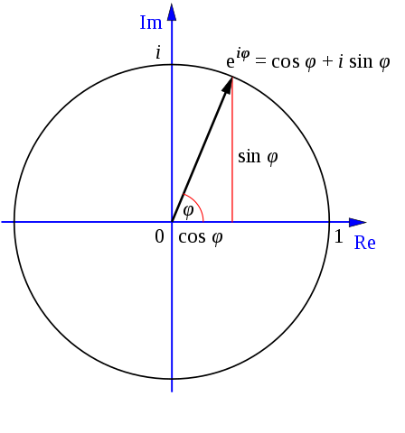
The Swiss mathematican Euler, not long after the concept of complex numbers came about, noticed a relationship between the dot moving along a unit circle and the way we express complex numbers. Here, one picture is worth a thousand words:
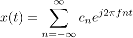
I promise you, I have not gone off on a tangent (no pun intended). The unit circle and projections collide in a vector space world to form possibly the most powerful tool in signal processing: Fourier series. Here's how: let's take a look at a periodic signal x(t) with period T. That signal, believe it or not, can be thought of as a vector in a signal space. Just like a vector space, we can find basis vectors to be mixed together to form x(t), and vice versa! To begin our hunt, notice what else have a period of T. That's right, our dot friend traversing along the unit circle. We can control its speed so that it travels along the unit circle in T, T/2, T/3, ... and so on. Even negative periods, which just means it will travel in the opposite direction. The slowest it will travel will be at T, and then it can speed up to form multiples of its base angular frequency, going \(\pm\)2*(2πf), \(\pm\)3*(2πf), \(\pm\)4*(2πf), and so on...
Using Euler's formula, we can combine the sin and the cos involved in describing the motion of the dot along the unit circle into a complex exponential, with period T (and f = 1/T), to have the following:
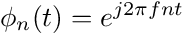
(We engineers use j to denote \(\sqrt{-1}\) because i is reserved for instantaneous current)
First, we make sure \(\phi_n(t)\) is actually periodic with period T. Let's see:
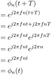
(Useful reminders: exponent rules, \(n\) is an integer, \(fT = 1\), and why does \(e^{j\pi n} \) equal to 1?)
Yes. \(\phi_n(t)\) for all integer values of n is periodic with period T (or faster fundamental periods in multiples of f), and the set {\(\phi_n(t)\)} for all integers n is the orthonormal set for the signal space where all signals x(t) are periodic with period T. Don't believe me? I'll let math show the way. Take two basis vectors in that set, say \(\phi_n(t)\) and \(\phi_m(t)\), what must happen when we project one vector onto another?
Yes, in other words, if n = m, so that the two vectors are actually the same, projecting the vector onto itself should give back 1, i.e. it takes one copy of the vector to make itself. Hopefully you see why. However, when n \(\neq\) m, we should get 0. No copies of \(\phi_n(t)\) can make \(\phi_m(t)\) if those are two different basis vectors, because they should be orthogonal!
Let's go:
Case 1: n = m
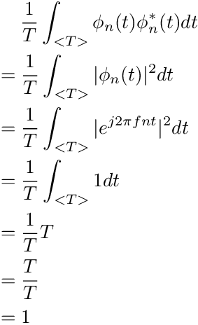
Here we make note of an important property of complex numbers in the above illustration that will come useful later. The product of a complex number and its conjugate is equal to the magnitude of the complex number squared. Of course, for the unit circle complex sinusoid, the magnitude is always 1, hence the 1 dt in the integrand in the middle steps.
Case 2: n =/= m
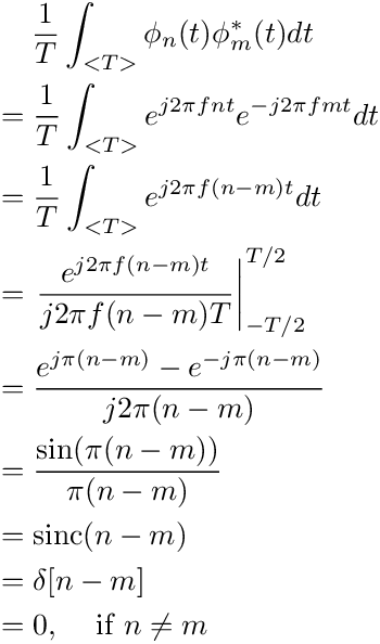
Here I delibrately introduced a few terms. First, I obtained sin from the complex sinusoid thanks to Euler's formula. Then, I got a fraction of sin()/(). The expressions involving sin()/() is so common in signal processing that there is a special name for such function, called "sinc", as in sinc(x) = sin(πx)/πx. For sin(0)/0, the limit goes to 1, so like a true engineer, we removed the discontinuity at that point and just assigned it value of 1. Next, remember that n and m's are integers, so unless they are the same, which would produce a value of 1, they would be 0 otherwise, since any integer multiples of π in argument of sin produces 0. This means sinc([n-m]) = δ[n-m], the Kronecker-delta functon, which equals to 1 if the argument is 0, and 0 in all other cases.
Right. It is pretty clear now that {\(\phi_n(t)\)} forms an orthonormal basis for the signal space where all signals in the space, x(t), is periodic with period T. This is how Fourier series is established.
Just as we can pick off the coordinates of a vector in R^2 Euclidean space to obtain the individual projections for each dimension, we can do the same for vectors in our signal space. We let "c_n" be the scalar multiple for the "nth" basis vector, \(\phi_n(t)\), where n is an integer, and we simply project the vector x(t) onto \(\phi_n(t)\) to obtain c_n, like so:
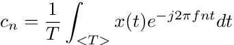
The above equation is called the "analysis equation", because we are projecting the signal onto a particular basis vector, to, well, analyze the signal in that component.
We'll talk about "c_n" later, but for now, let's see how we can get back x(t) by appropriately combining the basis vectors:
The above equation is called the "synthesis" equation because we are synthesizing the signal x(t) by combining scaled versions of the basis vectors. The nth basis vector has scalar multiple of "c_n". This is only possible because those basis vectors form an orthonormal set in the signal space.
There is another name for the synthesis equation: Fourier series, named after the French mathematician Joseph Fourier. What Fourier discovered was that if we combine different sinusoids with multiples of the base frequency of the signal, 1/T, we can represent any periodic signal with period T. The amount to combine for each sinusoid? Their corresponding Fourier coefficients, "c_n".
So for any periodic signal, its Fourier series representation can be thought of as adding up a bunch of vibrating strings, or "harmonics", vibrating at integer multiples of the base frequency. How much of a particular harmonic contributes to the original signal depend on the value of its corresponding Fourier coefficient.
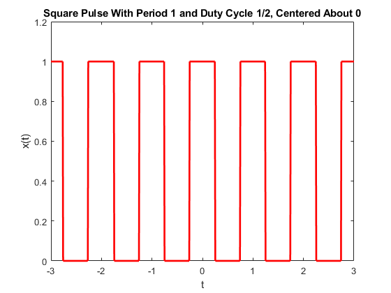
Let's do an example and find the Fourier series representation of a square wave. A square wave with period T is a signal that is 1 during a fraction of the time within one period T, and 0 in the other times in that period. The fraction of time in which the square wave is 1 (on) is called its "Duty Cycle", denoted as δ. So mathematically, the square wave has the following equation:
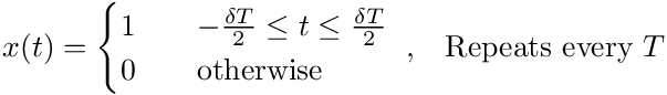
Here I conveniently shifted the square wave such that it is an even function. This will come in handy later on. As a visual guide with some concrete parameter values:
Let's apply the analysis equation to obtain the Fourier Coefficients. Please note that for c_0, we have:
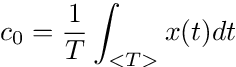
Which is just the average value of the signal over one period T, since the exponent of 0 is 1 for any non-zero base. Therefore, c_0 for our square wave is just δ, the duty cycle.
For non-zero n, c_n is more complicated but nonetheless very fascinating:
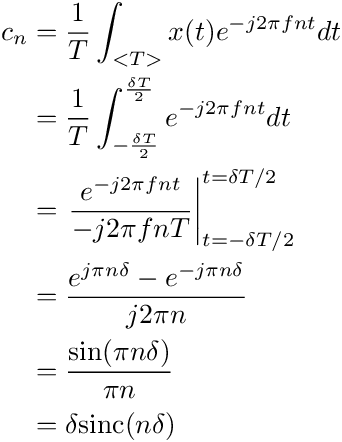
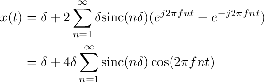
Please note that sinc is an even function, so c_(-n) = c_n, and putting everything together using the synthesis equation, we get:
In fact, it is not a coincidence that the Fourier coefficients of a real signal x(t) "fold" along the n = 0 axis, such that |c_(-n)| = |c_n|. Here, let me prove it.
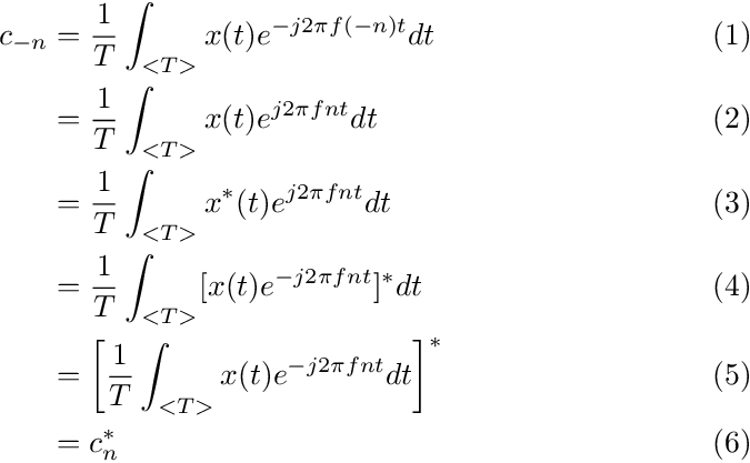
The first line is directly from the definition of the synthesis equation. Going from line 2 to line 3 I used the fact that x(t) is given to be real, so it is equal to its own conjugate. Lines 4 and 5 use the properties of complex numbers for conjugates and finally going from line 5 to line 6 we use the definition of the synthesis equation again.
The above result tells us that the non-zero Fourier coefficients of a real signal x(t) is conjugate symmetric about n = 0. If the Fourier coefficients are real, as we saw for the case of the square wave, then c_(-n) = c_n. In any case, the magnitude of c_(-n) is equal to the magnitude of c_n. This property will also come in handy later.
Thank you for making it all the way to this point. For doing so, you shall be handsomely rewarded. This section contains the punchline of this whole blog. Let me start by introducing the notion of average power to periodic signals. The average power of a signal, to put it plainly, is the total energy of that signal over the period of time considered. For a periodic signal, a nice time duration to consider is over one period of the signal (duh!). That's cool. Now what about energy? Well, for a real signal, the energy is the integral of the square of that signal over the desired time period. For a complex signal, it's the magitude squared.
So what about the power of a periodic signal x(t)? Well, let's find out if it has something to do with its Fourier coefficients.
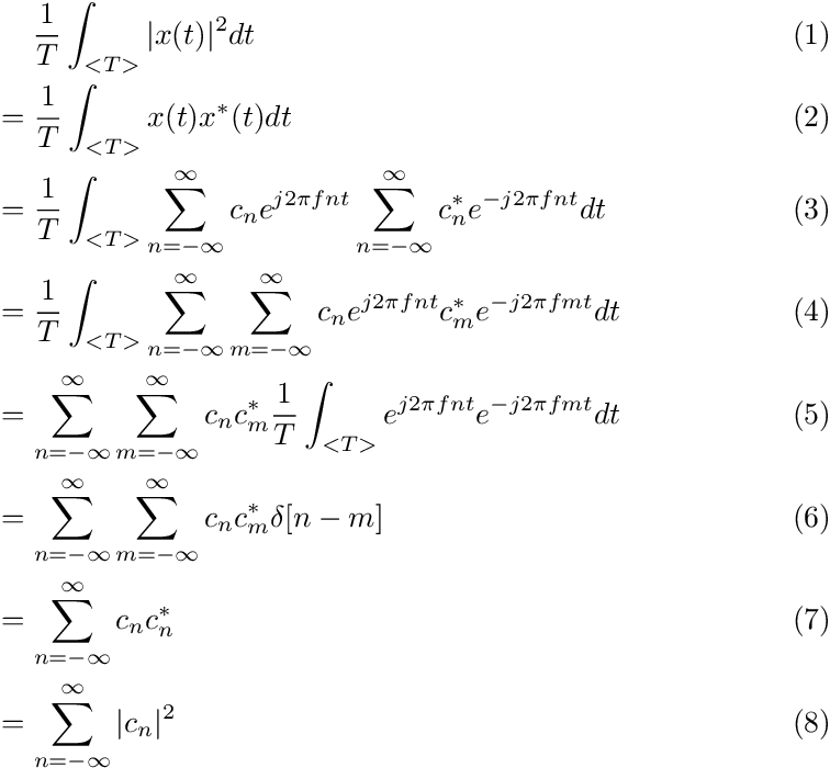
This one's a doozy, so let me explain carefully. The above is the proof of Parseval's Theorem, which states that the average power of a periodic signal x(t) with period T is equal to the sum of the magnitude squared of its Fourier coefficients. The first line is using the complex number property regarding the product of itself and its conjugate that I mentioned earlier. Then we apply the synthesis equation on both x(t) and its conjugate counterpart. Next, we combine the product of the two sums inside the integral as a double-summation. Then comes the part that works but if I were a mathematician, I would show that it works to be more rigorous. But...I'm an engineer. So I look at the integral which itself is a sum, and I switched it with the double sum on line 4 (which happens to be valid here mathematically). Then, realizing the integral is nothing but the projection of the nth basis vector onto the mth, we get the Kronecker-delta function for (n-m) which then collapses the double sum and then voila!
We can even combine our earlier result about the Fourier coefficients of a real signal being conjugate symmetric about n = 0 into Parseval's theorem, such that if x(t) were real, then:
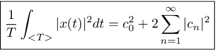
Please note that for c_0, it is the average value of the signal x(t) over one period T, so if x(t) is real, then so is c_0, and therefore we can simply square c_0.
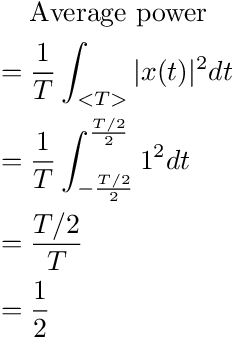
Now, let's have some fun! Let us apply Parseval's theorem to the square wave we were examining earlier and see what kind of results we get. We will do so by taking the average power of the square wave with period T and duty cycle 1/2 in two ways using Parseval's Theorem.
Direct definition:
Via Fourier coefficients:
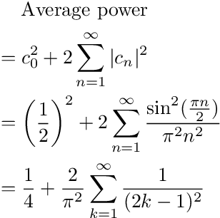
Please observe that for sin(πn/2), if n is even, then the argument in sine is an integer multiple of π, which would yield 0. This means c_n for all even n of a square wave is 0. For odd harmonics, it's \(\pm\) 1 in the numerator of c_n since it's either multiples of sin(π/2) or sin(3π/2). In any case, squaring the value will always yield 1.
By Parseval's theorem:
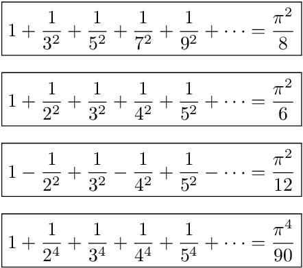
Wait...let me see that last line again...
One of the most fascinating series in mathematics...derived from Fourier series.
Having fun yet?
***
We don't stop here. Remember, Fourier series exist in all periodic signals. Square waves are boring, so let us spice things up with a quadratic function repeated every T = 2π. Yes, the quadratic f(t) = t^2. Like so:
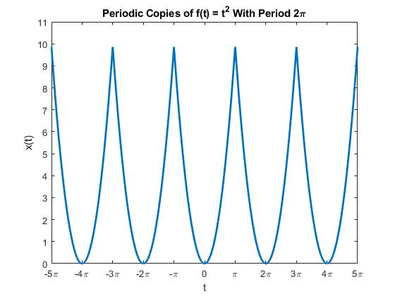
What I did was I took f(t) = t^2, and windowed it to the interval [-π, π]. Then, I simply let it repeat every 2π from minus to positive infinity.
The Fourier series representation of this repeated quadratic wave is as follows:
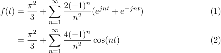
The Fourier coefficients are actually given in the first equation. The second equation makes the Fourier series more compact by collapsing the complex sinusoids into the cosine function via Euler's formula.
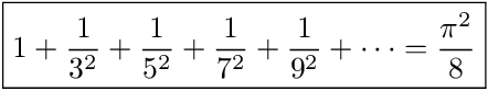
Now let's plug in some values for t. Let's see what happens when t = π. And remember, cos(nπ) = = (-1)^n for integer values of n. If you don't believe me, graph cosine function and see for yourself!
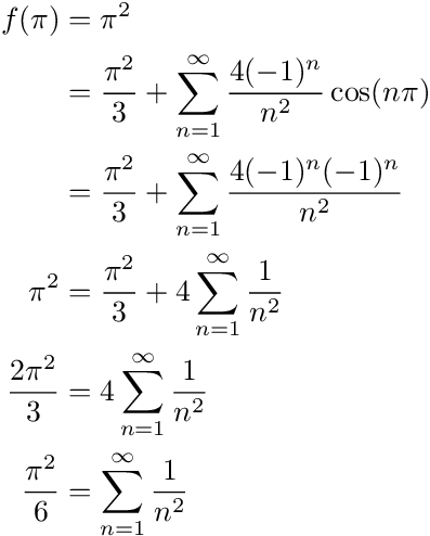
Wait...let me see that last line again...
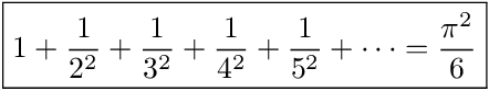
One of the most fascinating series in mathematics...derived from Fourier series.
Having fun yet?
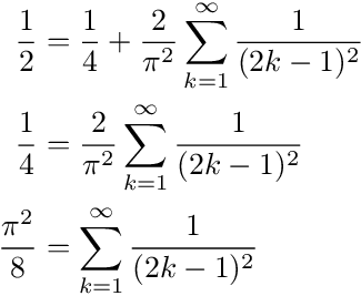
Now, let t = 0:
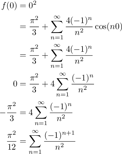
Wait...let me see that last line again...
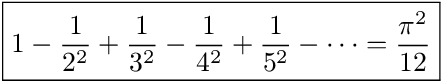
One of the most fascinating series in mathematics...derived from Fourier series.
Having fun yet?
But wait, there's more! We have not applied Parseval's Theorem on our lovely quadratic wave yet. Let's see what happens when we do that. For the average power of the wave:
Direct definition:
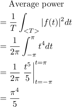
Via Fourier coefficients:
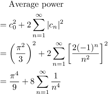
Applying Parseval's theorem, we get:
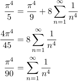
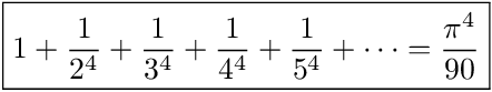
Wait...let me see that last line again...
Having fun yet?

Using Fourier series, any infinite sums of fraction powers can be shown to converge to some proprotion of π's powers; you just have to pick the right function, the right period, and decide whether to apply values from Fourier series itself or apply Parseval's theorem!
Having pie for lunch!