
May 30, 2023
Almost three years ago, I published an interesting tidbit that connected signal processing to math, and specifically, to the famous number \(\pi\). In that blog post, I revealed how Fourier Series are essentially recipes to create a cake made of periodic signals, and we can use the deconstruction of that cake to conclude that \(1 + 1/2^2 + 1/3^2 + 1/4^2 + \dots = \pi^2/6\). However, recently what compelled me to revisit the blog post is the emergence of some sudden philosophical musings on the interplay between engineering and math. You see, by no means is applying the Fourier Series a rigorous proof of the infamous equation mentioned above. I showed the derivation using Fourier Series three years ago because...maybe I was just too excited (or bored) at the time and figured that it was somewhat of an elegant revelation that I had to share with my readers. Of course, now that I am more mature, I realize that there are some more steps needed, mathematically, to prove the identity completely. Is this blog post about atoning the sin of rigor transgressed in that blog post of three years past? No. Instead, I am going to re-explain the derivation of the identity, using the same tools as that of the earlier blog post, and double down on why engineers use and "abuse" math for the sake of human progress.
The gist of engineering is to use models to provide solutions to physical problems in a scaled-down universe and give everyone the "I told you so" when the solution invariably works in the real universe. Those models are formed based on the laws of science and governed by the principles of math, but by no means are they required, nor are they in actuality, a replica of the real system the models try to represent. Statistician George Box worded it best: "All models are wrong, but some are useful."
The best example lies unbiasedly in signal processing, an area of engineering that I had the pleasure of studying for much of my university career. Remember how you yawned during math class when the teacher wrote down "\(i = \sqrt{-1}\)" on the chalkboard and called it an imaginary number? Walk a mile in my shoes and you will find out that in signal processing, it is weirder not to talk about \(i\), which by the way we actually denote as \(j\) since the former letter is reserved for instantaneous current (electricity). Indeed, when talking about signals, whether in time or in frequency domain, we assume the signal has complex values, and we go from there. Why, you might ask. The shortest answer I can provide you is that we model signals using complex numbers. Yes, we work with complex numbers, even though complex signals do not exist in our physical universe, because it is a wrong, but useful, model. For one thing, complex numbers carry two parts of information to one part for a real number: a complex number has a magnitude and an angle, which we can use to denote both the amplitude and the phase shift of real-world signals, something real numbers cannot do. In addition, for Fourier Series, instead of expressing basis functions in terms of both sine and cosine, we can skip trig altogether, use Euler's Formula and acknowledge the usefulness of complex numbers to express things in exponentials. One function, no trig, no hassles.
Here, in this blog post, I will show you how engineers "abuse" math to make math useful by re-deriving the \(1 + 1/2^2 + 1/3^2 + 1/4^2 + \dots = \pi^2/6\) equation using signal processing, which, remember, is not at all mathematically rigorous. I will call out, whenever I can, bits of mathematics in my derivation that will make mathematicians balk but engineers take for granted. And despite the latter, the sun will still rise the next day as life goes on.
We start with the notion of basis functions, which in my earlier blog post I called as "ingredients" to a cake. The recipe amount for each ingredient is determined by the analysis equation, which projects the cake onto that ingredient, and the output is a scalar number representing how much of that ingredient makes the cake. The set of ingredients, namely functions, form what is called a basis for the resulting signals. In signal processing, there are usually a countably infinite number of ingredients, but fret not, we can still make a yummy cake. By the way, as aptly named, the equation that combines the right amounts of ingredients to form the cake is called the synthesis equation.
The basis functions for a periodic signal of period \(T\) is the following:
\begin{align} \phi_n(t) &= \left\{\frac{e^{j\omega nt}}{\sqrt{T}}\right\}, \quad n = 0,\pm1, \pm2, \pm3, \dots \\ \end{align}
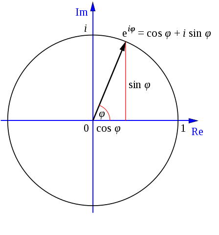
Remember \(j = \sqrt{-1}\) is our imaginary number. When it appears in the exponent, we have a complex sinusoid, which is an imaginary signal of complex value combining a sine wave and a cosine wave. The two waves are combined into the complex sinusoid thanks to Euler's Formula, and we never have to use sine and cosine in practice in signal processing. The \(\omega\) is the natural frequency of the periodic signal and is equal to \(\frac{2\pi}{T}\), as there are \(2\pi\) radians in a full revolution. By the way, this is where the "\(\pi\)" comes from our identity we are trying to prove.
(Euler's Formula in a nutshell)
Each \(n\) represents an ingredient, and here there are a countably infinite number of them. We can easily tell how much of one ingredient is needed via the analysis equation, but first, we must make sure that the basis functions are orthonormal. The importance of which I explained in my earlier blog post. Here, I just show it by projecting one basis onto another and see if the result is always 0 unless the two basis functions are the same, in which case the result should be 1.
We always model signals as vector spaces with defined inner products, which are a measure of how close two vectors are to each other component-wise. The inner product is defined as the sum of the products of each vector's components, with the first multiplying the complex conjugate of the latter, and where the sum becomes integration if the time domain is continuous. Remember, in signal processing, we model signals as complex by default, because it's wrong but useful.
Let the \(n\)th ingredient's amount be \(c_n\). We have:
\begin{align} c_n &= \int_{-\frac{T}{2}} ^ {\frac{T}{2}} \phi_n(t) \phi_m^*(t)\, \mathrm{d}t \\ \\ &= \int_{-\frac{T}{2}} ^ {\frac{T}{2}} \frac{e^{j\omega nt}}{\sqrt{T}} \frac{e^{-j\omega mt}}{\sqrt{T}}\, \mathrm{d}t \\ \\ &= \frac{1}{T}\int_{-\frac{T}{2}} ^ {\frac{T}{2}} e^{j\omega (n-m)t}\, \mathrm{d}t \\ \end{align}
Case 1: \(n = m\). In this case we have \(n - m = 0\) and so:
\begin{align} c_n &= \frac{1}{T}\int_{-\frac{T}{2}} ^ {\frac{T}{2}} e^{j\omega (n-m)t}\, \mathrm{d}t \\ \\ &= \frac{1}{T}\int_{-\frac{T}{2}} ^ {\frac{T}{2}} \, \mathrm{d}t \\ \\ &= \frac{T}{T} = 1\\ \end{align}
Case 2: \(n \neq m\). In this case we have \(n - m \neq 0\) and so:
\begin{align} c_n &= \frac{1}{T}\int_{-\frac{T}{2}} ^ {\frac{T}{2}} e^{j\omega (n-m)t}\, \mathrm{d}t \\ \\ &= \frac{1}{T}\left[\frac{e^{j\omega (n-m)t}}{j\omega (n-m)}\right]_{t = -\frac{T}{2}} ^ {t = \frac{T}{2}} \\ \\ &= \frac{1}{T}\left[\frac{e^{j\omega (n-m)(T/2)} - e^{-j\omega (n-m)(T/2)}}{j\omega (n-m)}\right] \end{align}
Recall that \(\omega = \frac{2\pi}{T}\), we have:
\begin{align} c_n &= \frac{1}{T}\left[\frac{e^{j\omega (n-m)(T/2)} - e^{-j\omega (n-m)(T/2)}}{j\omega (n-m)}\right] \\ \\ &= \frac{e^{j\pi(n-m))} - e^{-j\pi(n-m)}}{2j\pi(n-m)} \\ \\ &= \frac{\sin{[\pi (n-m)]}}{\pi (n - m)} \end{align}
Since \(n - m \neq 0\), first of all we are not dividing by zero, which is good. Second, since \(n\) and \(m\) are integers, the argument to the sine function is a multiple of \(\pi\), which means the value is always 0. This proves that:
\begin{align} \phi_n(t) &= \left\{\frac{e^{j\omega nt}}{\sqrt{T}}\right\}, \quad n = 0,\pm1, \pm2, \pm3, \dots \\ \end{align}
Is indeed an orthonormal basis to periodic signals with period \(T\).
The function \(f(t) = \frac{\sin{(\pi t)}}{\pi t}\) has a removable discontinuity at \(t = 0\), because the limit of \(f(t)\) as \(t\) approaches 0 exists and is equal to 1. When that happens, if we just assign the value \(f(0) = 1\), then we essentially make \(t = 0\) a continuous point for the function, effectively "removing" the discontinuity. When that happens, the function looks like this:
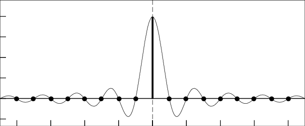
If you recognize this as the picture I placed in the "About Me" section, congratulations! I did so to reflect my proud background in signal processing. The above function, \(f(t) = \frac{\sin{(\pi t)}}{\pi t}\), is so ubiquitous in signal processing that engineers there gave it a special name, the "sinc function", pronounced as "sink". Actually, the sinc function exists in the math realm too, but engineers made two adjustments. First, the input is scaled by \(\pi\) so that the zeros of the function is always at integer values of \(t\), and second, and possibly the more egregious alternation, is that it is simply defined as:
\begin{align} \text{sinc}(t) &:= \frac{\sin(\pi t)}{\pi t} \end{align}
That's it. No cases to consider, nothing. It's a function that has zeros only where \(t\) is a non-zero integer, and at \(t = 0\), it has the value of 1. This is a moment where the mathematician will object defiantly, "But the function is undefined at \(t = 0\) !". Relax, engineers know better, but by "removing" that removable discontinuity makes the expression much more efficient to, well, express. Looking at this, then we don't even need to divide our orthonormal proof from earlier into cases. Simply,
\begin{align} c_n &= \frac{1}{T}\int_{-\frac{T}{2}} ^ {\frac{T}{2}} e^{j\omega (n-m)t}\, \mathrm{d}t \\ \\ &= \text{sinc}[\pi (n - m)] \\ \\ &= \delta_{nm} \end{align}
Remember the above sinc function is a discrete-time signal with time index \((n - m)\). Since it's scaled by \(\pi\), it's value is 1 when \(n = m\) and 0 otherwise, which is exactly the definition of the Kronecker delta on the last line above. One case, no hassles.
All right, so to recap, if we have an orthonormal basis \(\{\phi_n(t)\}\) spanning the vector space of periodic signals with period \(T\), and hence \(\omega = \frac{2\pi}{T}\), our analysis equation to find how much of \(n\)th ingredient contribute to the signal \(x(t)\) in the vector space is:
\begin{align} c_n &= \int_{-\frac{T}{2}} ^ {\frac{T}{2}} x(t) \phi_n^*(t)\, \mathrm{d}t \\ \end{align}
And putting the cake together by their ingredients in the right amounts is our synthesis equation:
\begin{align} x(t) &= \sum_{n = -\infty}^{\infty} c_n \phi_n(t) \\ \end{align}
If we use the orthonormal basis that we just proved for periodic signals into \(\phi_n(t)\), we have the following equations.
Analysis equation:
\begin{align} c_n &= \frac{1}{T} \int_{-\frac{T}{2}} ^ {\frac{T}{2}} x(t) e^{-j\omega nt}\, \mathrm{d}t \\ \end{align}
Synthesis equation:
\begin{align} x(t) &= \sum_{n = -\infty}^{\infty} c_n e^{j\omega nt}\\ \end{align}
"But wait just a minute!", the mathematician once again protested passionately, "What happened to the \(\sqrt{T}\,\) in the orthonormal basis functions??? Without it, \(c_n\) are not the right ingredient amounts!"
"Calm down", the engineer replied, "we just had to make sure the basis functions are orthogonal so we don't get cross-contamination of ingredients for our cake. It's okay if the analysis equation is off by a factor of \(\sqrt{T}\), as long as the synthesis equation is off by a factor of \(1/\sqrt{T}\), which is what we have here."
"Plus", the engineer added, "by doing so, the analysis equation looks more natural, as if we are integrating over one period and dividing by the length of that period. The synthesis equation is also compact without having to carry the \(1/\sqrt{T}\) as a fraction."
"But the \(c_n\)'s are not the right values for the orthonormal basis!", the mathematician argued loudly.
"But your cell phone still works", the engineer said calmly.
In that earlier blog post for part 1, I showed and proved Parseval's Theorem. I am going to do it again, but pointing out where the mathematician would start to object, and explain why that is okay.
In layman terms, Parseval's Theorem equates the power of a periodic signal in time domain to that in its frequency domain, the latter being in Fourier Series form. The theorem states that:
\begin{align} \frac{1}{T}\int_{-\frac{T}{2}} ^ {\frac{T}{2}} |x(t)|^2\, \mathrm{d}t &= \sum_{n = -\infty}^{\infty}|c_n|^2 \\ \end{align}
Let's prove it!
\begin{align} \text{L.H.S} &= \frac{1}{T}\int_{-\frac{T}{2}} ^ {\frac{T}{2}} |x(t)|^2\, \mathrm{d}t \\ \\ &= \frac{1}{T}\int_{-\frac{T}{2}} ^ {\frac{T}{2}} x(t) x*(t)\, \mathrm{d}t \\ \\ &= \frac{1}{T}\int_{-\frac{T}{2}} ^ {\frac{T}{2}} \sum_{n = -\infty}^{\infty} c_n e^{j\omega nt} \left(\sum_{n = -\infty}^{\infty} c_n e^{j\omega nt}\right)^*\, \mathrm{d}t \\ \\ &= \frac{1}{T}\int_{-\frac{T}{2}} ^ {\frac{T}{2}} \sum_{n = -\infty}^{\infty} c_n e^{j\omega nt} \sum_{n = -\infty}^{\infty} c_n^* e^{-j\omega nt}\, \mathrm{d}t \\ \\ &= \frac{1}{T}\int_{-\frac{T}{2}} ^ {\frac{T}{2}} \sum_{n = -\infty}^{\infty} \sum_{m = -\infty}^{\infty} c_n c_m^* e^{j\omega nt} e^{-j\omega mt}\, \mathrm{d}t \\ \\ &= \sum_{n = -\infty}^{\infty} \sum_{m = -\infty}^{\infty} c_n c_m^* \left[\frac{1}{T}\int_{-\frac{T}{2}} ^ {\frac{T}{2}} e^{j\omega nt} e^{-j\omega mt}\, \mathrm{d}t \right] \\ \\ &= \sum_{n = -\infty}^{\infty} \sum_{m = -\infty}^{\infty} c_n c_m^* \delta_{nm} \\ \\ &= \sum_{n = -\infty}^{\infty} c_n c_n^* \\ \\ &= \sum_{n = -\infty}^{\infty} |c_n|^2 = \text{R.H.S} \end{align}
Q.E.D
Except, it's not Q.E.D, because in the middle I swapped the order of summation and integration and placed the latter to the innermost layer. While swapping orders for summations are fine mathematically, swapping integration is generally not a good idea to please a mathematician because integrals are continuous summations. This means that while one can treat an integral as a summation, it is actually a limit since it deals with continuity. The swapping caused the integration to change, which means we must show in the newer case that the limit still exists, and so on.
However, in signal processing, swapping integrals with summations and other integrals is very commonplace and forms a quick way to show not only Parseval's Theorem, but key concepts such as convolution in the time domain being equivalent to multiplication in the frequency domain. This quick proof led to the concept of phasors in circuit analysis, as convolutions are very expensive, and dare I say convoluted, way of computing things. A mathematician can express displeasure however they like, but as one engineer said, "your cell phone still works, and that's the standard I abide by."
In part 1, I showed the Fourier Series for the following square wave:
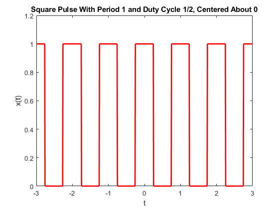
A square wave has two parameters: 1) its period, \(T\), and its duty cycle, \(\delta\), a real number between 0 and 1 describing the percentage of time in a period where the wave is "on", i.e. attaining the value of 1, vs. when it's "off", attaining the value of 0. Therefore, a square wave of period \(T\) and duty cycle \(\delta\) is the following function:
\begin{align} x(t) &= \begin{cases} 1, \quad -\frac{\delta T}{2} \leq t \leq \frac{\delta T}{2}\\ \\ 0, \quad \text{otherwise} \\ \end{cases}, \quad \text{repeats every } T \\ \end{align}
I trust my readers can apply the analysis equation to obtain the Fourier Series coefficients of the above square wave, so I will just reveal the answer below. It is:
\begin{align} c_n &= \begin{cases} \delta, \quad \text{if } n = 0 \\ \\ \frac{\sin(\pi n \delta)}{\pi n} , \quad \text{if } n \neq 0 \\ \end{cases} \end{align}
Which can also be succinctly written as \(c_n = \delta\, \text{sinc} (\delta n)\).
If we apply Parseval's Theorem here, we can express the power of the square wave in two ways. Let's consider \(\delta = 1/2\), i.e. a 50% duty cycle. Then, in the time domain, we have:
\begin{align} \text{Power} &= \frac{1}{T}\int_{-\frac{T}{2}} ^ {\frac{T}{2}} |x(t)|^2\, \mathrm{d}t \\ \\ &= \frac{T/2}{T} = \frac{1}{2} \\ \end{align}
In the frequency domain, we have:
\begin{align} \text{Power} &= \sum_{n = -\infty}^{\infty}|c_n|^2 \\ \\ &= \left(\frac{1}{2}\right)^2 + 2\sum_{n = 1}^{\infty} \left(\frac{\sin(\pi n/2)}{\pi n} \right)^2 \\ \\ &= \left(\frac{1}{2}\right)^2 + 2\sum_{n = 1, \, n \text{ odd}}^{\infty} \frac{1}{\pi^2 n^2} \\ \\ &= \frac{1}{4} + \frac{2}{\pi^2} \sum_{n = 1, \, n \text{ odd}}^{\infty} \frac{1}{n^2} \\ \end{align}
Equating the two equations, we have:
\begin{align} \frac{1}{2} &= \frac{1}{4} + \frac{2}{\pi^2} \sum_{k = 1}^{\infty} \frac{1}{(2k-1)^2} \\ \\ \frac{1}{4} &= \frac{2}{\pi^2} \sum_{k = 1}^{\infty} \frac{1}{(2k-1)^2} \\ \\ \frac{\pi^2}{8} &= \sum_{k = 1}^{\infty} \frac{1}{(2k-1)^2} \\ \end{align}
That is,
\begin{align} 1 + \frac{1}{3^2} + \frac{1}{5^2} + \frac{1}{7^2} + \dots &= \frac{\pi^2}{8} \\ \end{align}
The equation above by itself is already pretty neat, but we can go further. Our holy grail is \(1 + 1/2^2 + 1/3^2 + 1/4^2 + \dots\), so let's just call that value \(x\). We can see our equation from above being part of the holy grail expression, and we just have to look at the even terms in the denominator. That is:
\begin{align} &\frac{1}{2^2} + \frac{1}{4^2} + \frac{1}{6^2} + \frac{1}{8^2} + \dots \\ \\ &= \left(\frac{1}{4}\right) \left(1 + \frac{1}{2^2} + \frac{1}{3^2} + \frac{1}{4^2} + \dots \right) \\ \\ &= \left(\frac{1}{4}\right) x \end{align}
Putting everything together, we have:
\begin{align} x &= \left(\frac{1}{4}\right) x + \frac{\pi^2}{8} \\ \\ \left(\frac{3}{4}\right) x &= \frac{\pi^2}{8} \\ \\ x &= \left(\frac{\pi^2}{8}\right)\left(\frac{4}{3}\right) \\ \\ x &= \frac{\pi^2}{6} \\ \end{align}
That is,
\begin{align} 1 + \frac{1}{2^2} + \frac{1}{3^2} + \frac{1}{4^2} + \dots &= \frac{\pi^2}{6} \\ \end{align}
It is quite satisfying for me, as an engineer, to see that even though we apparently cut corners by "abusing" math to achieve solutions, nonetheless based on math, at an extraordinary pace, the blissfulness that math provides from time to time can still be dug up by the very field that exploits it.
(No mathematicians were harmed in the making of this blog post.)