
May 31, 2020
In my previous blog post "The Chosen One", I discussed how math makes sense of everything by being consistent: independent derivations of answers to problems arrive at, well, the same answers. The problem that I described was with regards to the probability that you would be the sole survivor in a Pubg match. Assuming there are N players equally skilled, the probability that you would be the sole survivor is the same as the guy next to you in the lobby: 1/N.
But being stuck inside and playing a lot more Pubg Mobile than I should recently has taught me one thing: nope, not all players are equally skilled. The probability that you would be the chosen one drastically changes if we assign a specific probability of you winning a fight based on your skill level, as compared to your opponents. In the real world where I need much practice to be the best, what is my probability of being the sole survivor? Well, in a small celebration of me achieving Diamond ranking in Season 13 of Pubg Mobile after much ups and downs, I will find the answer for you right now.

***
We cannot use symmetry anymore to get a straightforward answer. Since not all players are equally skilled now, the only intuition we have is that players who are highly skilled should have a higher probability of becoming the sole survivor than as compared to those lower skilled. In order to proceed mathematically, we recall the stochastic chart from part 1.
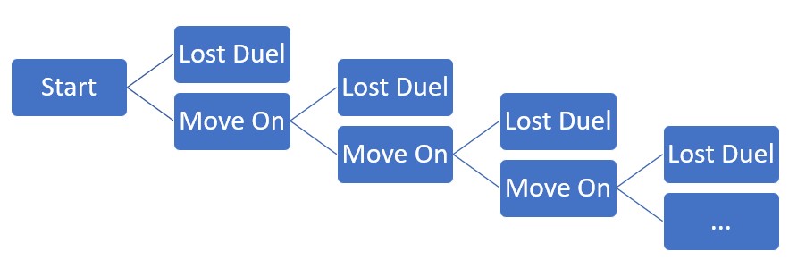
In our model, we simulate a Pubg match as a duel-selection duel-matchup process whereby you become the sole survivor if you win every duel that you get selected to participate. There will be N-1 duels in a matchup with N players, as each duel eliminates exactly one player. If you survive N-1 rounds, either by not getting picked or winning the duel if you get selected, then you are the sole survivor. Any slip-ups along the way and it's better luck next time.
Now, if we try to derive a mathematical expression for the conditional probability, things would start to get really, really messy, as we cannot just evaluate the probability of you getting selected for the duel at stage k as being (k-1)/(k choose 2) as seen in part 1. This is because it now matters who your opponent is. If you get selected to duel with the top-ranked player in the arena that is not you, you would be less likely to win than if you get matched with the worst player.
Okay, so now what do we do? Well, it is 2020 after all, and we have something at our disposal called "computers". We will rely on it to give us an empirical result on the distribution of winning counts of players. In order to do so, we need to extend our model to account for player skills.
Consider N players in a Pubg match. We will rank each player based on skill level, with the first player being the top-ranked player in the arena, second player being the second-rank, and so on, until the Nth player being the worst-ranked player. The players participate in the match using the duel-selection duel-matchup process shown in the stochastic chart. When two players (k, j) get matched (where k and j are their rankings, respectively), the probability that the kth player would win the duel is given by:
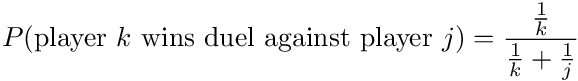
The above model is inspired by the Zipf Distribution, which is a probability distribution often associated with the frequency of occurrences of words in a language. It states that the frequency of occurrence of words in any language is inversely proportional to its ranking. For example, the word "the" is the most common English word, followed by "be" (and its conjugations). Therefore, in a body of work such as a novel, the word "be" would appear about half as often as "the". Similarly, the third most common English word, "to", would appear 1/3 as often as "the", and as 2/3 as often as "be". In similar spirits, if you are the top ranked player going up against the second-ranked player, it is nature to think that the second ranked player would be about half as likely to win against its top-ranked opponent. This is achieved with the above model of duel winning probability.
Now it's time to make our computers work. Computers, in general, are pretty obtuse objects that are capable of calculating very quickly, but most of the time they don't do unless as told. We rely on software installed on computers to get the machine to do something useful. Fortunately, we do have a piece of software, called Matlab, that is quite capable of telling the computer to simulate our mode of not-equally-skilled matchup of N players in a Pubg arena. Let me walk you through the setup.
%% Start of Simuation
N = 100; % Number of Participants
winningCount = zeros(N, 1);
simCount = 1e5;

for k = 1:simCount
soleSurvivor = getWinningPlayer(N);
winningCount(soleSurvivor) = winningCount(soleSurvivor) + 1;
fprintf('Simulation %d done!\n', k);
end

%% Display in Histogram
figure;
bar(winningCount./sum(winningCount));
title('Bar Graph of Number of Times Each Player is the Sole Survivor');
xlabel('Player');
ylabel('Sole Survivor Count / Total Matches Simulated');
Pretty simple it seems, doesn't it? I simulate the Pubg Mobile matchup 100,000 times, and each time, the winning player is generated using the model described above, and is packaged inside the function "getWinningPlayer(N)". After the simulation completes, I display the players' winning counts in a bar graph normalized against the total number of matches simulated.
After 100,000 simulations of Pubg Mobile matches of ranked players, what have we got? Well, please see the graph below:
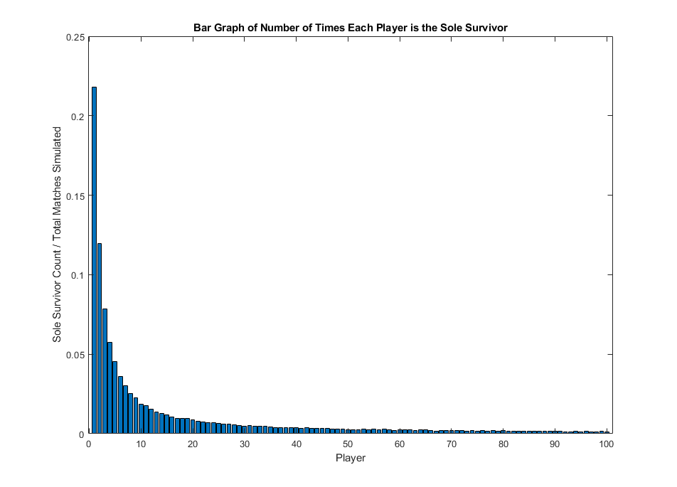
It appears that the top-ranked player wins twice as often as compared to the second-ranked, three times as often as compared to the third-ranked, four times as often as compared to the fourth-ranked, and so on. In other words, the winning counts for the players in a ranked arena of N players follow a Zipf Distribution! From the Zipf Distribution we get the 80-20 rule: if we add up the total winnings for the top 20%-ranked players, we get a total number of winnings equal to:
>> sum(winningCount(1:20))

ans =

   77025
Since we simulated the Pubg matches 100,000 times, the answer is 77% of all matches. In other words, we got a situation that in a ranked arena, the top 20%-ranked players win about 80% of all the matches!
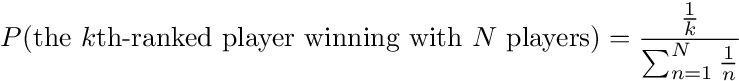
In the end, if you are the kth-ranked player in a Pubg match with N players, where k is between 1 and N, inclusive, then the probability of you winning the match would be:
***
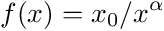
But hold on to your horses for just a moment. Let us fit a Pareto curve, which is the continous analog of the Zipf Distribution, with paremeter α = log(5)/log(4) that would generate the 80-20 rule (see Epilog of this blog for more details), to the bar graph above. The curve we would fit in this case would be approximately:
We get the following:
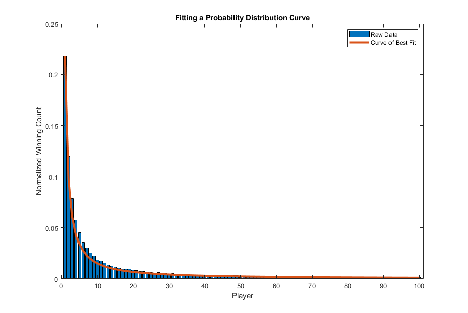
Remember, the only thing that we differed in our model as compared to part 1 was that we let the duel winning probability to be based on players' ranks, as opposed to 1/2 for the equally-skilled case. And yet, what emerged is a result that adheres to the 80-20 rule: the players' winning counts are distributed in a Zipf Distribution, with about 80% of all of the simulated matches won by just the top 20% of ranked players. This is the beauty of math, and why it was picked up by humans to help describe the universe we live.
The complete Matlab simulation codes can be found on my github account:
Where did the 80-20 rule arise? In this section, I will help readers digest where it came from and why it was so prevalent.
The 80-20 rule is associated with the Italian Economist Vilfredo Pareto, who discovered while studying income inequality that about 80% of the wealth in a population is often held by just 20% of the population. He further quantified this observation with his famous Pareto Distribution. In this distribution, the frequency of occurrences, say wealth, is inversely proportional to one's rankings. The richest individual would own approximately 2n times as much wealth as the second-richest, and 3n times as much as the third-richest, and so on, where n is based on a variable parameter. When n = 1, the parameter value α is log(5)/log(4) and we get the 80-20 rule.
To see this, we need to consider the CDF of the Pareto Distribution of type-α, which is:
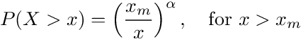
Here "x" represents a specific ranking in a population, and P(X > x) represents the probability that a random variable X exceeds the threshold given by x. In other words, P(X > x) represents the proportion of the population that is making above x amount of money, where x_m is the minimum income considered in the distribution, say. In our income example, saying that 20% of the population owns 80% of the wealth means that the probability of P(X > income in the top 20th percentile) = 1/5.
What constitutes a percentile? Well, if we are giving the minimum value x_m, to which everyone makes above that amount (so x_m is the 0th percentile), then on a scale, we can show the 80th percentile as follows:
At the very left side of the first green block, we have x_m. The red block represents wealth from 4x_m to infinity, and represents the top 20% of earners. So to find the α corresponding to the 80-20 rule, we need to find P(X > 4x_m) and set it to 1/5. I.e. The top 20% of owners horde 80% of all the wealth.
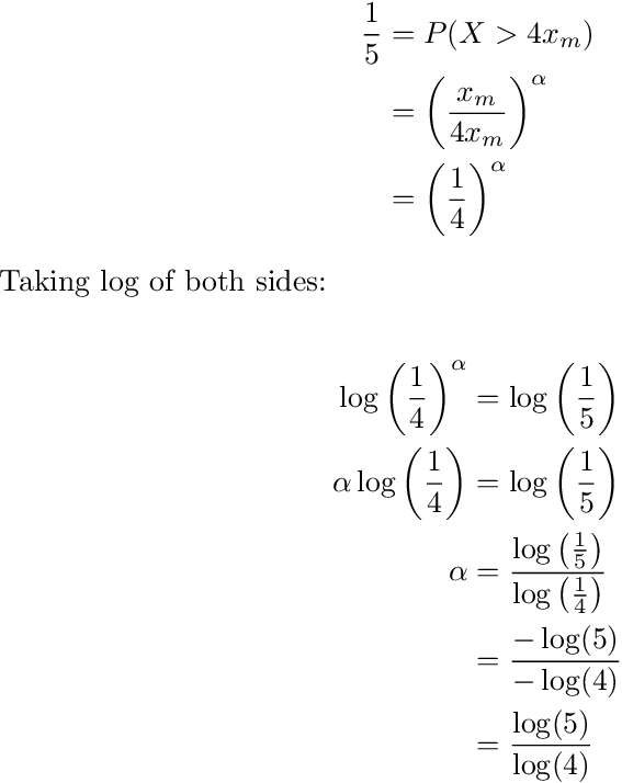
Note: the above derivation does not prove the 80-20 rule. It simply derives the value of α, known as the Pareto Index, that yields the 80-20 rule under Pareto Distribution. The 80-20 rule remains a common observation in our society.
Which brings me to the next point: why is it so prevalent? Well, we know that the 80-20 rule is a consequence of Pareto Distribution, which essentially states ones rankings are inversely proportional to ones wealth. So equivalently, we ask ourselves why this is the case. The truth is that there are no definite answers to this, but ultimately, this could be caused by a known snowball-effect: the rich gets richer. The reason for exponential growth--having stuff that makes more stuff, e.g. money, is why if you are the richest person in a population set, you will be well-equipped to make more money, and over time, be twice as rich as the second richest, and so on. And when such patterns emerge, we arrive at a Pareto Distribution that emerges the 80-20 rule. The discrete case of this is the Zipf Distribution, as seen in our ranked Pubg Mobile match simulation.