
August 18, 2024
Let's consider two real functions: \(f(x) = x^x\) and \(f(x) = x^{-x}\). For both of those two functions, let's consider for \(x > 0\). What the two functions are representing is exponential growth and decay, respectively, that scales with the base. Clearly, as \(x\) grows to infinity, the value of the first function approaches infinity while the value of the second approaches 0. What is interesting, however, is the dynamic when \(x\) is between 0 and 1. That is what the Bernoulli integral is depicting:
\begin{align} \int_{0}^{1} x^x \,\mathrm{d}x \end{align}
Along with its cousin:
\begin{align} \int_{0}^{1} x^{-x} \,\mathrm{d}x \end{align}
This is what this blog post is going to explore. Let's start with \(f(x) = x^x\).
In order to evaluate the Bernoulli integral, it's best to visualize our goal. This starts with plotting the function in which we are to calculate the area under its curve. Instead of plugging the function in a computer software, it's more insightful to do this the old-fashioned way.
Domain: \(\{x > 0\}\).
End-behaviors: \(\lim\limits_{x \to \infty} x^x = \infty\)
For \(\lim\limits_{x \to 0^+} x^x\), it's better to write the function as \(e^{\log{x^x}} = e^{x \log{x}}\), where \(\log\) is the natural logarithm. Since the exponential function is continuous, we can simply look at how the exponent is going to converge, if it does.
\begin{align} &\lim\limits_{x \to 0^+} x \log{x} \\ \\ =& \lim\limits_{t \to \infty} \frac{\log{(1/t)}}{t} \\ \\ =& \lim\limits_{t \to \infty} \frac{-t}{t^2} \quad \text{(L'Hôpital's rule)} \\ \\ =& \lim\limits_{t \to \infty} \frac{-1}{t} \\ \\ =& 0 \end{align}
And hence \(\lim\limits_{x \to 0^+} x^x = \lim\limits_{x \to 0^+} e^{x \log{x}} = e^0 = 1\).
Therefore, there is a removable discontinuity for \(f(x) = x^x\) at \((0, 1)\), and also note that \(f(1) = 1\). So the function starts with a value of 1 at \(x = 0\) and returns to 1 again when \(x = 1\). So what goes on for \(x\) between 0 and 1? Let's keep going to find out.
Critical Points: We need to find the first derivative of \(f(x) = x^x\).
Again, write \(x^x\) as \(e^{\log{x^x}} = e^{x \log{x}}\). Then, take the derivative of \(e^{x \log{x}}\):
\begin{align} &(e^{x \log{x}})' \\ \\ =& e^{x \log{x}} (\log{x} + 1) \quad \text{(Chain rule, product rule)}\\ \\ =& x^x (\log{x} + 1) \end{align}
Setting \(f'(x) = 0\), we see that since \(x^x\) is always greater than 0, we need to have \(\log{x} + 1 = 0\), or \(\log(x) = -1\). Solving for \(x\), we have \(x^* = e^{-1}\) as the sole critical point of the function.
Inflection points: we need to find the second derivative of \(x^x\):
\begin{align} &(x^x)'' \\ \\ =& [(e^{x \log{x}})']'\\ \\ =& (e^{x \log{x}} (\log{x} + 1))'\\ \\ =& e^{x \log{x}} (\log{x} + 1)^2 + e^{x \log{x}}(1/x) \quad \text{(product rule)} \\ \\ =& e^{x \log{x}} ((\log{x} + 1)^2 + 1/x) \\ \\ =& x^x ((\log{x} + 1)^2 + 1/x) \end{align}
Since \(x > 0\), then \(x^x\), \((\log{x} + 1)^2\), and \(1/x\) are all greater than 0. This means that \(x^x\) has NO inflection points and is always concave up. This also means that the critical point \(x^* = e^{-1} \approx 0.37\) is also where the global minimum for the function resides, and that global minimum is \((1/e)^{(1/e)} \approx 0.69\).
We now have all the information we need to plot \(x^x\), as seen below:
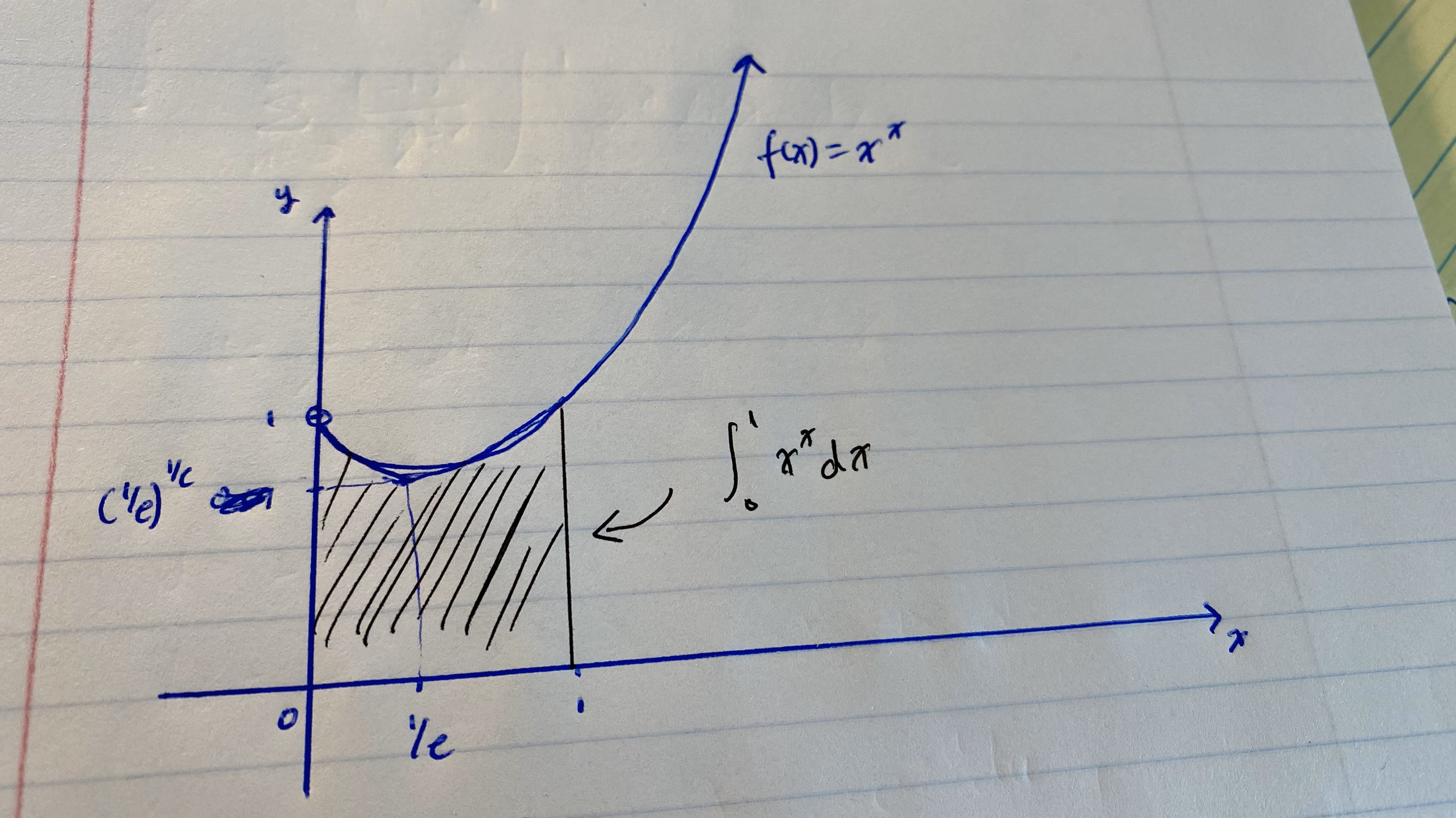
Summary: concave up (like the \(x^2\) parabola) with critical point at \((1/e, (1/e)^{(1/e)})\) as the global minimum, starts at (0, 1) as a removable discontinuity and grows to infinity. The area under the curve between \(x = 0\) and \(x = 1\) is our Bernoulli integral in which we are trying to evaluate. Clearly, the integral should be less than \(1 \times 1 = 1\).
The gamma function, denoted as \(\Gamma(z)\), is a complex function conceived by the Swiss mathematician Daniel Bernoulli that is key to evaluating the Bernoulli integral (hence the name of the integral!). It is basically a function that was the result of a task assigned to Bernoulli, asking him: how can we interpolate the factorial operation \(n! = n \times (n - 1) \times (n - 2) \times \dots 1\) for whole number values of \(n\) to the complex number world? Bernoulli said, "leave it to me!", and he came up with:
\begin{align} \Gamma(z) &= \int_{0}^{\infty} t^{z-1}e^{-t} \,\mathrm{d}t \end{align}
From a cursory glance we see that the exponential decay in \(t\) dominates the polynomial growth in \(t\), and hence the integral converges for any values of \(z\) where the real part of \(z\) is greater than 0. Then, the function is analytically extended to cover the entire complex plane, as complex functions often do. However, we don't need to worry about that. Let us simply check to see if Bernoulli did his homework correctly by verifying that the gamma function actually interpolates the factorial. Namely, we need to verify that:
\begin{align} \Gamma(n) &= (n - 1)! \quad \text{for } n = 1, 2, 3, \dots \end{align}
For this, we can use induction. The base case is \(n = 1\). Here, we have:
\begin{align} \text{L.H.S} &= \Gamma(1) \\ \\ &= \int_{0}^{\infty} t^{1-1}e^{-t} \,\mathrm{d}t \\ \\ &= \int_{0}^{\infty} e^{-t} \,\mathrm{d}t \\ \\ &= e^0 - e^{-\infty} \\ \\ &= 1 = 0! = \text{R.H.S} \end{align}
Now we can set up the induction hypothesis: let \(\Gamma(k) = (k - 1)!\) for any positive integer \(k\). Let us evaluate \(\Gamma(k + 1)\):
\begin{align} &\Gamma(k + 1) \\ \\ =& \int_{0}^{\infty} t^{k + 1 -1}e^{-t} \,\mathrm{d}t \\ \\ =& \int_{0}^{\infty} t^{k}e^{-t} \,\mathrm{d}t \\ \end{align}
Integration by parts gives us: \(u = t^k\), \(\mathrm{d}u = kt^{k - 1}\mathrm{d}t\), \(\mathrm{d}v = e^{-t} \,\mathrm{d}t\), \(v = -e^{-t}\)
\begin{align} &\Gamma(k + 1) \\ \\ =& \int_{0}^{\infty} t^{k}e^{-t} \,\mathrm{d}t \\ \\ =& uv|_{t = 0}^{\infty} - \int_{0}^{\infty} v \, \mathrm{d}u \\ \\ =& -t^k e^{-t} |_{t = 0}^{\infty} + \int_{0}^{\infty} kt^{k - 1}e^{-t} \,\mathrm{d}t \\ \\ =& k \int_{0}^{\infty} t^{k - 1}e^{-t} \,\mathrm{d}t \quad \text{(The first term goes to 0)} \\ \\ =& k (k - 1)! \quad \text{(By our induction hypothesis)} \\ \\ =& k! \end{align} As desired.
Therefore, it turns out Bernoulli did his homework correctly, as the gamma function successfully interpolates the factorial.
Now we have everything we need to evaluate the Bernoulli integral. Let's start:
\begin{align} &\int_{0}^{1} x^{x} \,\mathrm{d}x \\ \\ =& \int_{0}^{1} e^{x \log{x}} \,\mathrm{d}x \\ \\ =& \int_{0}^{1} \sum_{k = 0}^{\infty} \frac{(x \log{x})^k}{k!} \,\mathrm{d}x \\ \\ &\text{(Taylor series expansion of } e^x \text{about } x = 0 \text{)}\\ \\ =& \sum_{k = 0}^{\infty}\frac{1}{k!} \int_{0}^{1} x^k \log^k{x} \,\mathrm{d}x \\ \end{align}
If we were to use the gamma function to help us evaluate the integral, we need to set the bounds of integration to go from 0 to \(\infty\). Currently, we have the bounds going from 0 to 1, so we make the u-substitution \(x = e^{-u}\) to make the change happen. As \(u \to \infty\), \(e^{-u} \to 0\), and \(e^{-0} = 1\), so this works. Here, \(\mathrm{d}x = -e^{-u}\,\mathrm{d}u\).
\begin{align} &\sum_{k = 0}^{\infty}\frac{1}{k!} \int_{0}^{1} x^k \log^k{x} \,\mathrm{d}x \\ \\ =& \sum_{k = 0}^{\infty}\frac{1}{k!} \int_{\infty}^{0} e^{-uk} (-u)^k (-e^{-u})\,\mathrm{d}u \\ \\ =& \sum_{k = 0}^{\infty}\frac{(-1)^k}{k!} \int_{0}^{\infty} e^{-uk} u^k (e^{-u})\,\mathrm{d}u \\ \\ =& \sum_{k = 0}^{\infty}\frac{(-1)^k}{k!} \int_{0}^{\infty} u^k e^{-(k+1)u}\,\mathrm{d}u \\ \\ \end{align}
Now, we are very close to getting the integral to mimic that of a gamma function. However, there are still a couple of things that are different. For start, notice the exponent on \(u\) is \(k\) where as in the gamma function, it's \(z - 1\), and so we make a dummy variable substitution in the outer summation, letting \(m = k + 1\) and hence \(k = m - 1\).
\begin{align} &\sum_{k = 0}^{\infty}\frac{(-1)^k}{k!} \int_{0}^{\infty} u^k e^{-(k+1)u}\,\mathrm{d}u \\ \\ =& \sum_{m = 1}^{\infty}\frac{(-1)^{m - 1}}{(m - 1)!} \int_{0}^{\infty} u^{m - 1} e^{-mu}\,\mathrm{d}u \\ \\ \end{align}
We are almost done. Now, we just need to make the \(-mu\) term in the exponent into just a single \(-t\), so we make that substitution, letting \(t = mu\). Hence, \(\mathrm{d}t = m\,\mathrm{d}u\).
\begin{align} &\sum_{m = 1}^{\infty}\frac{(-1)^{m - 1}}{(m - 1)!} \int_{0}^{\infty} u^{m - 1} e^{-mu}\,\mathrm{d}u \\ \\ =& \sum_{m = 1}^{\infty}\frac{(-1)^{m - 1}}{(m - 1)!} \int_{0}^{\infty} \left(\frac{t}{m}\right)^{m - 1} e^{-t} \left(\frac{1}{m}\right)\,\mathrm{d}t \\ \\ =& \sum_{m = 1}^{\infty}\frac{(-1)^{m - 1} m^{-m}}{(m - 1)!} \int_{0}^{\infty} t^{m - 1} e^{-t}\,\mathrm{d}t \\ \end{align}
Now we have gotten the gamma integral, which equals to \((m - 1)!\) for every positive integer \(m\). Therefore, we finish off with:
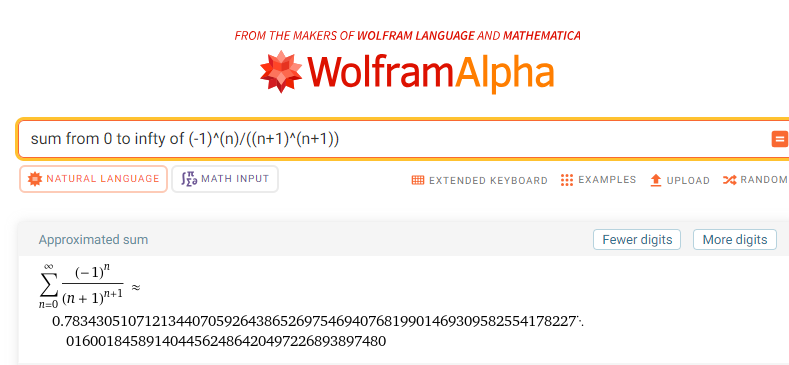
\begin{align} &\sum_{m = 1}^{\infty}\frac{(-1)^{m - 1} m^{-m}}{(m - 1)!} \int_{0}^{\infty} t^{m - 1} e^{-t}\,\mathrm{d}t \\ \\ =& \sum_{m = 1}^{\infty}\frac{(-1)^{m - 1} m^{-m}}{(m - 1)!} (m - 1)! \\ \\ =& \sum_{m = 1}^{\infty}\frac{(-1)^{m - 1}}{m^{m}} \\ \\ =& \sum_{n = 0}^{\infty}\frac{(-1)^{n}}{(n + 1)^{n + 1}} \approx 0.78\\ \end{align}
Where in the last line I just changed the summation to start at 0, if some people prefer zero-based.
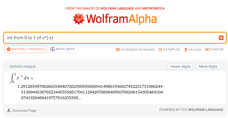
Let's now check the result with Wolfram Alpha:
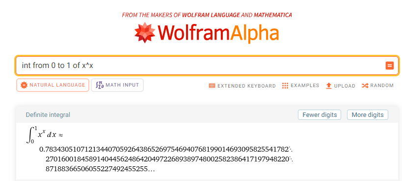
We have successfully evaluated the Bernoulli integral. Now, let's explore its cousin, \(f(x) = x^{-x}\).
Again, we use the same manual analysis for plotting the function \(f(x) = x^{-x}\).
Domain: \(\{x > 0\}\).
End-behaviors: \(\lim\limits_{x \to 0^+} x^{-x} = 1\), \(\lim\limits_{x \to \infty} x^{-x} = 0\)
Again, there is a removable discontinuity for \(f(x) = x^{-x}\) at \((0, 1)\).
Critical Points: We need to find the first derivative of \(f(x) = x^{-x}\).
Again, write \(x^{-x}\) as \(e^{\log{x^{-x}}} = e^{-x \log{x}}\). Then, take the derivative of \(e^{-x \log{x}}\):
\begin{align} &(e^{-x \log{x}})' \\ \\ =& e^{-x \log{x}} (-\log{x} - 1) \quad \text{(Chain rule, product rule)}\\ \\ =& - x^{-x} (\log{x} + 1) \end{align}
Setting \(f'(x) = 0\), we see that since \(x^{-x}\) is always greater than 0, we need to have \(\log{x} + 1 = 0\), or \(\log(x) = -1\). Solving for \(x\), we have \(x^* = e^{-1}\) as the sole critical point of the function.
Inflection points: we need to find the second derivative of \(x^{-x}\):
\begin{align} &(x^{-x})'' \\ \\ =& (-e^{-x \log{x}} (\log{x} + 1))'\\ \\ =& e^{-x \log{x}} (\log{x} + 1)^2 - e^{-x \log{x}}(1/x) \quad \text{(product rule)} \\ \\ =& e^{-x \log{x}} ((\log{x} + 1)^2 - 1/x) \\ \\ =& x^{-x} ((\log{x} + 1)^2 - 1/x) \end{align}
Unlike the case with \(f(x) = x^x\), here the second derivative of \(x^{-x}\) can be 0, if \(((\log{x} + 1)^2 - 1/x) = 0\). Solving this equation for \(x\) yields \(x = 1\) (can be solved by inspection). Hence, there is one inflection point for \(f(x) = x^{-x}\) at \(x = 1\).
Here, we need to do some critical thinking. We know that the function starts at 1 and returns to 1 for \(x\) between 0 and 1. There is one critical point at \(x^* = e^{-1} \approx 0.37\). There is only one inflection point at \(x = 1 > e^{-1}\). Therefore, at \(x^* = e^{-1}\), the point must be a global maximum and for \(x < 1\), the curve is concave down. For \(x > 1\), the curve is concave up the rest of the way.
We now have all the information we need to plot \(x^{-x}\), as seen below:
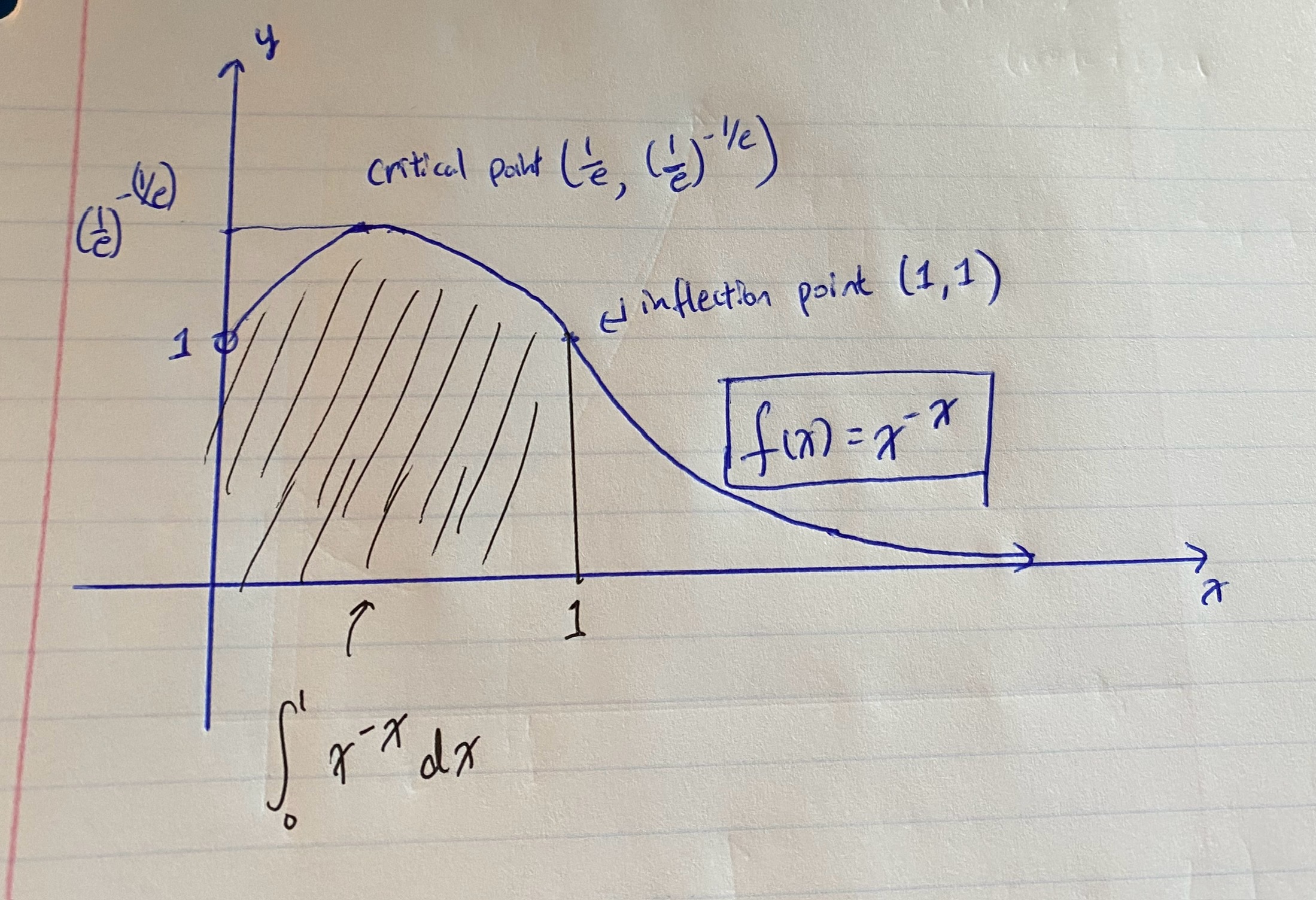
Summary: concave down for \(x < 1\) and concave up for \(x > 1\) with critical point at \((1/e, (1/e)^{-(1/e)} \approx 1.44)\) as the global maximum, starts at (0, 1) as a removable discontinuity but decays to 0. The area under the curve between \(x = 0\) and \(x = 1\) is our Bernoulli integral's cousin in which we are trying to evaluate. Clearly, the integral should be greater than \(1 \times 1 = 1\).
The process to evaluate the cousin of the Bernoulli integral is similar to that for the Bernoulli integral and makes use of the gamma function. Let's see if you can follow along!
\begin{align} &\int_{0}^{1} x^{-x} \,\mathrm{d}x \\ \\ =& \int_{0}^{1} e^{-x \log{x}} \,\mathrm{d}x \\ \\ =& \int_{0}^{1} \sum_{k = 0}^{\infty} \frac{(-x \log{x})^k}{k!} \,\mathrm{d}x \\ \\ =& \sum_{k = 0}^{\infty}\frac{(-1)^k}{k!} \int_{0}^{1} x^k \log^k{x} \,\mathrm{d}x \\ \\ =& \sum_{k = 0}^{\infty}\frac{(-1)^k}{k!} \int_{\infty}^{0} e^{-uk} (-u)^k (-e^{-u})\,\mathrm{d}u \\ \\ =& \sum_{k = 0}^{\infty}\frac{(-1)^k (-1)^k}{k!} \int_{0}^{\infty} u^k e^{-(k+1)u}\,\mathrm{d}u \\ \\ =& \sum_{k = 0}^{\infty}\frac{1}{k!} \int_{0}^{\infty} u^k e^{-(k+1)u}\,\mathrm{d}u \\ \\ =& \sum_{m = 1}^{\infty}\frac{1}{(m - 1)!} \int_{0}^{\infty} u^{m - 1} e^{-mu}\,\mathrm{d}u \\ \\ =& \sum_{m = 1}^{\infty}\frac{1}{(m - 1)!} \int_{0}^{\infty} \left(\frac{t}{m}\right)^{m - 1} e^{-t} \left(\frac{1}{m}\right)\,\mathrm{d}t \\ \\ =& \sum_{m = 1}^{\infty}\frac{m^{-m}}{(m - 1)!} \int_{0}^{\infty} t^{m - 1} e^{-t}\,\mathrm{d}t \\ \\ =& \sum_{m = 1}^{\infty}\frac{m^{-m}}{(m - 1)!} (m - 1)! \\ \\ =& \sum_{m = 1}^{\infty} m^{-m} \approx 1.29\\ \end{align}
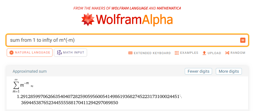
We get, perhaps, a result even more elegant than the Bernoulli integral itself:
\begin{align} \int_{0}^{1} x^{-x} \,\mathrm{d}x = \sum_{m = 1}^{\infty} m^{-m} \\ \end{align}